Construct a basis of principal balances for a compositional data set.
pb_basis(
  X,
  method,
  constrained.criterion = "variance",
  cluster.method = "ward.D2",
  ordering = TRUE,
  ...
)
Arguments
- X
Compositional data set.
- method
Method used to construct the principal balances. One of `"exact"`, `"exact2"`, `"constrained"`, or `"cluster"`.
- constrained.criterion
Criterion used by the constrained method. Either `"variance"` (default) or `"angle"`.
- cluster.method
Linkage criterion passed to
hclustwhen `method = "cluster"`.- ordering
Logical; if `TRUE`, reorder balances by decreasing explained variance.
- ...
Additional arguments passed to
hclust.
Value
A matrix whose columns are principal balances.
Details
Several methods are available:
`"exact"`: exact computation of principal balances,
`"exact2"`: exact computation using incremental Gray-code updates,
`"constrained"`: constrained approximation based on a target criterion,
`"cluster"`: approximation based on hierarchical clustering.
References
Martín-Fernández, J. A., Pawlowsky-Glahn, V., Egozcue, J. J., & Tolosana-Delgado, R. (2018). Advances in Principal Balances for Compositional Data. Mathematical Geosciences, 50, 273–298.
Examples
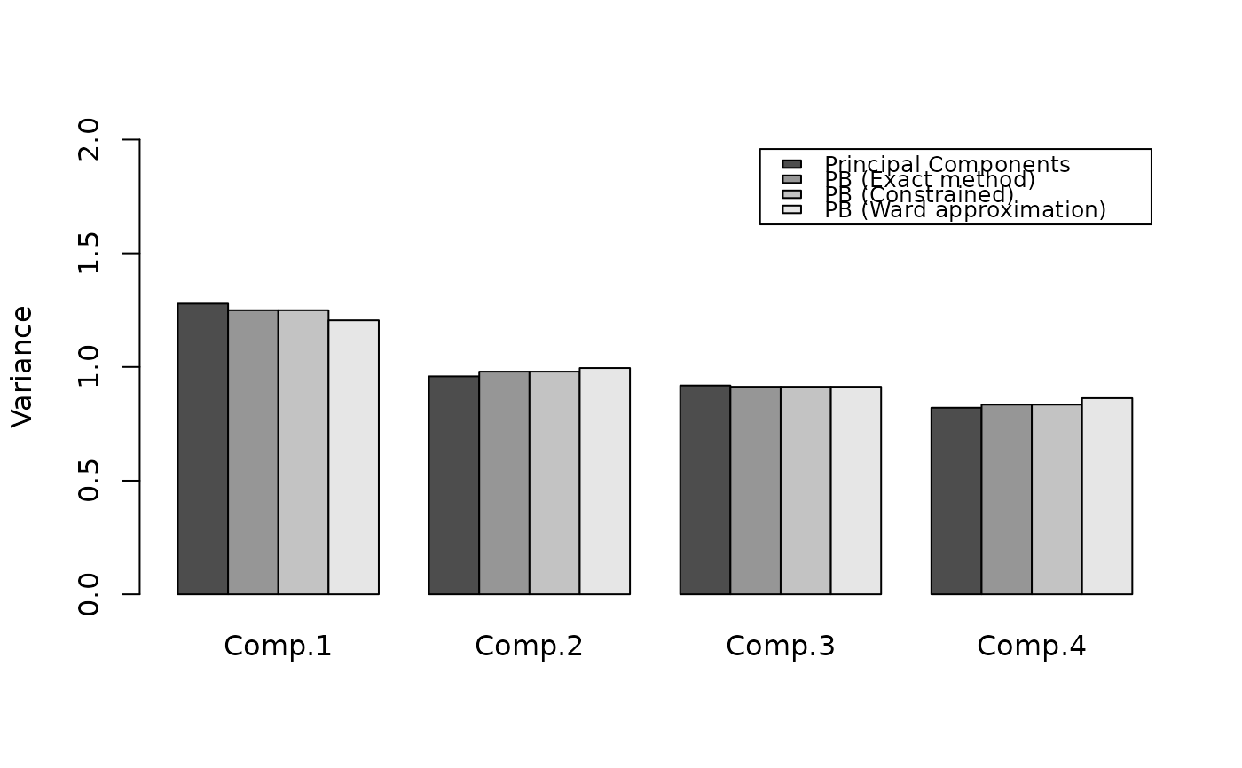
set.seed(1)
X <- matrix(exp(rnorm(5 * 100)), nrow = 100, ncol = 5)

v1 <- apply(coordinates(X, "pc"), 2, var)
v2 <- apply(coordinates(X, pb_basis(X, method = "exact")), 2, var)
v3 <- apply(coordinates(X, pb_basis(X, method = "constrained")), 2, var)
v4 <- apply(coordinates(X, pb_basis(X, method = "cluster")), 2, var)

barplot(
  rbind(v1, v2, v3, v4),
  beside = TRUE,
  ylim = c(0, 2),
  legend = c(
    "Principal Components",
    "PB (Exact method)",
    "PB (Constrained)",
    "PB (Ward approximation)"
  ),
  names = paste0("Comp.", 1:4),
  args.legend = list(cex = 0.8),
  ylab = "Variance"
)